Joshua Burton

PhD in Mathematical Biology, team member at PlantingSpace, software developer, general purpose AI systems and Bayesian inference researcher.

Posterior predictive checking with Turing and ArviZ, using the golf putting case study

The golf putting case study in the Stan documentation is a really nice showcase of iterative model building in the context of MCMC. In this post I'm going to demonstrate how the models in the Stan tutorial can be implemented with Turing, a Julia library for general-purpose probabilistic programming. This has already been done by Joshua Duncan^[1], so additionally I'll show how to make use of the ArviZ.jl package in order to do some posterior predictive analysis, specifically PSIS-LOO cross validation and LOO-PIT predictive checking. These are really powerful tools which can be used to help us evaluate our model fit, but I'll focus only on the implementation with Turing and ArviZ, so if you want to understand these tools and how to interpret them you can read about PSIS-LOO here, and LOO-PIT in Gelman et al. BDA (2014), Section 6.3.

For full details on each of the models, I suggest reading the case study in the Stan documentation, which is really nicely written and easy to follow.

Data visualisation
Models
Model selection
Conclusion
References

Data visualisation

The first thing to do is have a look at the data we have and see if we get any inspiration for a model.

using Turing, DelimitedFiles, StatsPlots, StatsFuns, ArviZ
gr(size=(580,301))

# Turing can have quite verbose output, so I'll
# suppress that for readability
# It's usually a good idea to not do this,
# so you are warned of any divergences
import Logging
Logging.disable_logging(Logging.Warn); # or e.g. Logging.Info

data = readdlm("_assets/blog/golf-putting-in-turing/code/golf_data_old.txt")
x, n, y = data[:,1], data[:,2], data[:,3];
yerror = sqrt.(y./n .* (1 .-y./n)./n)

scatter(x,y ./ n, yerror = yerror,
        ylabel = "Probability of success",
        xlabel = "Distance from hole (feet)",
        title = "Data on putts in pro golf",
        legend=:false,
        color=:lightblue,
        )

The error bars associated with each point $j$ in the plot are given by $\sqrt{\hat{p}_j(1−\hat{p}_j)/n_j}$ , where $\hat{p}_j=y_j/n_j$ is the success rate for putts taken at distance $x_j$ .

We can see a pretty clear trend – the greater the distance from the hole, the lower the probability of the ball going in.

Models

It's typically a good idea to start with a very simple model, and then slowly add in more features to improve the fit of our models. This is exactly what is done in the Stan documentation. One of the simplest models we can use in this instance is a logistic regression.

📝 I'll go through all of the details for defining the model, fitting it, and doing posterior checks in this first example, but in the later ones I'll just show the code and end result.

Logistic regression

The first model considers the probability of success (i.e. getting the ball in the hole) as a function of distance from the hole, using a logistic regression:

y_j \sim \text{Binomial}(n_j, \text{logit}^{-1}(a + bx_j)), \hspace{1em}\text{for j = 1,\dots, J.}

In Turing, this looks like

@model function golf_logistic(x, y, n)
    a ~ Normal(0,1)
    b ~ Normal(0,1)

    p = logistic.(a .+ b .* x)
    for i in 1:length(n)
        y[i] ~ Binomial(n[i],p[i])
    end
end

golf_logistic (generic function with 2 methods)

Fitting the model

We can fit this model with the No-U-Turn sampler (NUTS) using Turing's sample function.

logistic_model = golf_logistic(x,y,n)
fit_logistic = sample(logistic_model,NUTS(),MCMCThreads(),2000,4)

Chains MCMC chain (2000×14×4 Array{Float64, 3}):

Iterations        = 1001:1:3000
Number of chains  = 4
Samples per chain = 2000
Wall duration     = 0.84 seconds
Compute duration  = 0.81 seconds
parameters        = a, b
internals         = lp, n_steps, is_accept, acceptance_rate, log_density, hamiltonian_energy, hamiltonian_energy_error, max_hamiltonian_energy_error, tree_depth, numerical_error, step_size, nom_step_size

Summary Statistics
  parameters      mean       std      mcse    ess_bulk    ess_tail      rhat   ess_per_sec
      Symbol   Float64   Float64   Float64     Float64     Float64   Float64       Float64

           a    2.2222    0.0587    0.0013   2114.3991   2521.2274    1.0004     2620.0733
           b   -0.2548    0.0067    0.0001   2197.5697   2834.3650    1.0010     2723.1347

Quantiles
  parameters      2.5%     25.0%     50.0%     75.0%     97.5%
      Symbol   Float64   Float64   Float64   Float64   Float64

           a    2.1069    2.1817    2.2223    2.2607    2.3401
           b   -0.2680   -0.2594   -0.2548   -0.2503   -0.2416

Here we've computed 8000 posterior samples across 4 chains. The MCSE of the mean is 0 to two decimal places for both parameters, and both $\hat{R}$ values are close to 1, indicating convergence and good mixing between chains. So let's have a look at the fit.

Visualising the fit

The following plot shows the model fit. The black line corresponds to the posterior median, and the grey lines show 500 draws from the posterior distribution.

# get posterior median
meda, medb = [quantile(Array(fit_logistic)[:,i],0.5) for i in 1:2]

# select some posterior samples at random
n_samples = 500
fit_samples = Array(fit_logistic)
idxs = sample(axes(fit_samples,1),n_samples)
posterior_draws = fit_samples[idxs,:]

posterior_data = [logistic.(posterior_draws[i,1] .+ posterior_draws[i,2].*x) for i in 1:n_samples]
plot(x,posterior_data,color=:grey,alpha=0.08,legend=:false)

plot!(x,logistic.(meda .+ medb.*x),color=:black,linewidth=2)
scatter!(x,y ./ n, yerror = yerror,
        ylabel = "Probability of success",
        xlabel = "Distance from hole (feet)",
        title = "Fitted logistic regression",
        legend=:false,
        color=:lightblue)

A by-eye evaluation leads us to conclude this isn't a very good fit. Can we formalise this conclusion with some more rigorous tools?

Evaluating the fit using ELPD

The expected log pointwise predictive density (ELPD) is a measure of predictive accuracy for each of the $J$ data points taken one at a time^[2]. It can't be computed directly, but we can estimate it with leave-one-out (LOO) cross-validation. The LOO estimate of the ELPD can be noisy under certain conditions, but can be improved with Pareto smoothed importance sampling. This is the estimate implemented in ArviZ. In order to use the tools in ArviZ we first have to compute the posterior predictive distribution, save the pointwise log likelihoods from our model fit, and convert our Turing chains into an ArviZ InferenceData object.

📝 For our predictive posterior we replace the data y with a vector of missing values, similar(y, Missing).

# Instantiate the predictive model
logistic_predict = golf_logistic(x,similar(y, Missing),n)
posterior_predictive = predict(logistic_predict, fit_logistic)


# Ensure the ordering of the loglikelihoods matches the ordering of `posterior_predictive`
loglikelihoods = pointwise_loglikelihoods(logistic_model, fit_logistic)
names = string.(keys(posterior_predictive))
loglikelihoods_vals = getindex.(Ref(loglikelihoods), names)

# Reshape into `(nchains, nsamples, size(y)...)`
loglikelihoods_arr = permutedims(cat(loglikelihoods_vals...; dims=3), (2, 1, 3));

# construct idata object
idata_logistic = from_mcmcchains(
    fit_logistic;
    posterior_predictive=posterior_predictive,
    log_likelihood=Dict("ll" => loglikelihoods_arr),
    library="Turing",
    observed_data=(; x, n, y)
);

With this InferenceData object we can utilise some powerful analysis and visualisation tools in ArviZ.

For example, we can now easily estimate the ELPD with PSIS-LOO.

logistic_loo = loo(idata_logistic,pointwise=true);
println("LOO estimate is ",round(logistic_loo.elpd_loo[1],digits=2), " with an SE of ",round(logistic_loo.se[1],digits=2),
        " and an estimated number of parameters of ",round(logistic_loo.p_loo[1],digits=2))

LOO estimate is -204.31 with an SE of 62.58 and an estimated number of parameters of 39.4

The estimate itself is relative, so it isn't very useful in isolation, but we can see that the standard error is high, and the estimated number of parameters in the model is ~40, much larger than the true value of 1, indicating severe model misspecification.

Another tool at our disposal is the PSIS-LOO probability integral transform. Oriol Abril has written a nice blog post on how to interpret the following plots^[3], and I'll quote directly from the post to give some intuition about this:

Probability Integral Transform stands for the fact that given a random variable $X$ , the random variable $Y = F_X(X) = P(x\leq X)$ is a uniform random variable if the transformation $F_X$ is the Cumulative Density Function (CDF) of the original random variable $X$ . If instead of $F_X$ we have $n$ samples from $X$ , $\{x_1,\dots, x_n\}$ , we can use them to estimate $\hat{F}_X$ and apply it to future $X$ samples $x^*$ . In this case, $\hat{F}_X(x^∗)$ will be approximately a uniform random variable, converging to an exact uniform variable as $n$ tends to infinity.

So we're looking for our computed $\hat{F}_X$ to be, more or less, a uniform random variable. Anything other than this suggests that the model is a poor fit.

📝 This is not to say that if $\hat{F}_X$ is uniform then our model is good. Doing a large number of varied diagnostic checks, e.g $\hat{R}$ , ESS (bulk and tail), MCSE, and posterior predictive checks like PSIS-LOO, simply gives us more opportunity to identify any issues with our model.

The LOO-PIT for our simple logistic regression model is clearly not uniform which suggests to us, as expected, the model is a poor choice.

plot_loo_pit(idata_logistic; y="y")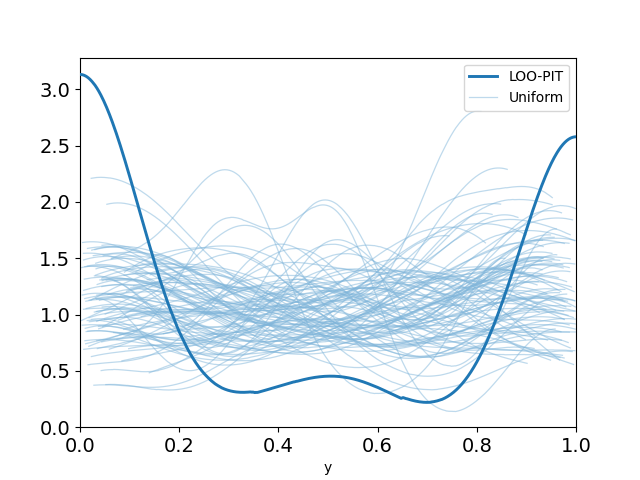

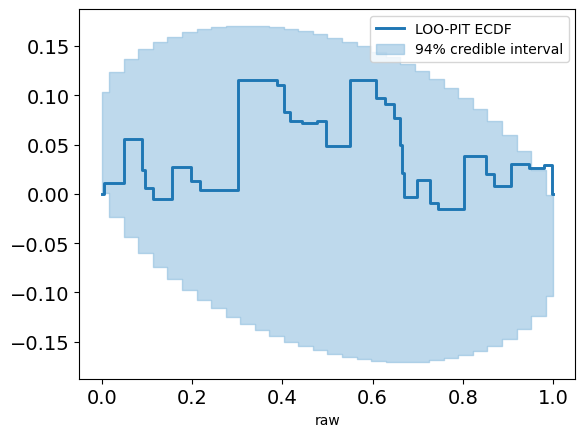
Sometimes it's not very clear if the estimate is non-uniform, so we can plot the difference between the LOO-PIT Empirical Cumulative Distribution Function (ECDF) and the uniform CDF instead of LOO-PIT kde for a more 'zoomed in' look.

plot_loo_pit(idata_logistic; y="y",ecdf=true)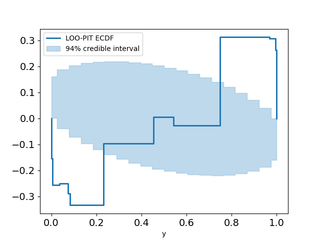

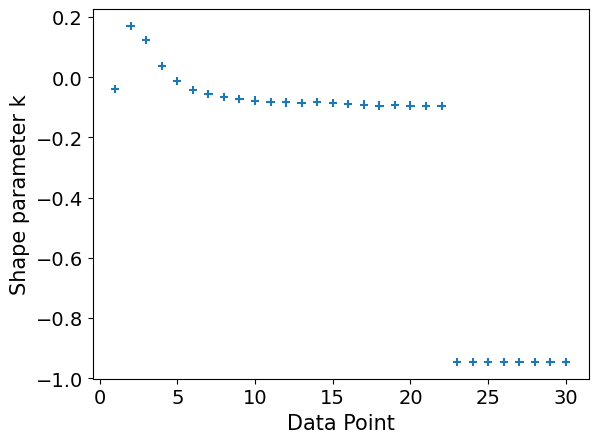
Lastly, it's a good idea to plot our Pareto $k$ diagnostic, to assess the reliability of the above estimates^[4]. In short, we're looking for values of $k < 0.7$ . Any $k$ values greater than 1 and we can't compute an estimate for the Monte Carlo standard error (SE) of the ELPD. In this case the ELPD estimate is not reliable. These high $k$ values also explain the large estimate for the effective number of parameters.

plot_khat(logistic_loo)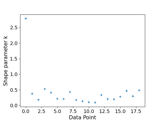

Modelling from first principles

So hopefully we're pretty convinced by now that this isn't a good model. An alternative approach is to consider the angle of the shot, where 0 corresponds to the centre of the hole. We assume that the golfers attempt to hit the ball directly at the hole (i.e. an angle of 0), but are not always perfect due to a number of (known or unknown) factors, so that the angle is Normally distributed about 0 with some standard deviation $\sigma$ . The model is derived in detail in the Stan documentation, so I will just show the Turing implementation.

Phi(x) = cdf(Normal(),x)

@model function golf_angle(x,y,n,r,R)
    threshold_angle = asin.((R-r) ./ x)
    sigma ~ truncated(Normal(0,1),0,Inf)
    p = 2 .* Phi.(threshold_angle ./ sigma) .- 1
    for i in 1:length(n)
        y[i] ~ Binomial(n[i],p[i])
    end
    return sigma*180/π # generated quantities
end

r = (1.68 / 2) / 12;
R = (4.25 / 2) / 12;

angle_model = golf_angle(x,y,n,r,R)
fit_angle = sample(angle_model,NUTS(),MCMCThreads(),2000,4)

Chains MCMC chain (2000×13×4 Array{Float64, 3}):

Iterations        = 1001:1:3000
Number of chains  = 4
Samples per chain = 2000
Wall duration     = 4.32 seconds
Compute duration  = 3.88 seconds
parameters        = sigma
internals         = lp, n_steps, is_accept, acceptance_rate, log_density, hamiltonian_energy, hamiltonian_energy_error, max_hamiltonian_energy_error, tree_depth, numerical_error, step_size, nom_step_size

Summary Statistics
  parameters      mean       std      mcse    ess_bulk    ess_tail      rhat   ess_per_sec
      Symbol   Float64   Float64   Float64     Float64     Float64   Float64       Float64

       sigma    0.0267    0.0004    0.0000   3327.7659   5156.3438    1.0026      857.0090

Quantiles
  parameters      2.5%     25.0%     50.0%     75.0%     97.5%
      Symbol   Float64   Float64   Float64   Float64   Float64

       sigma    0.0259    0.0264    0.0267    0.0269    0.0275

The model is fit just as before, and if we visualise the fit against the posterior median of the previous model it seems to be a lot better.

# get posterior median
med_sigma = quantile(Array(fit_angle),0.5)

# select posterior samples at random
n_samples = 500
fit_samples = Array(fit_angle)
idxs = sample(1:length(fit_angle),n_samples)
posterior_draws = fit_samples[idxs]

threshold_angle = asin.((R-r) ./ x)

post_lines = [2 .* Phi.(threshold_angle ./ posterior_draws[i]) .- 1 for i in 1:n_samples]
plot(x,post_lines,color=:grey,alpha=0.08,legend=:false)
plot!(x,2 .* cdf.(Normal(),threshold_angle ./ med_sigma) .- 1,color=:blue,linewidth=1.5)

plot!(x,logistic.(meda .+ medb.*x),color=:black,linewidth=2)
annotate!(12,0.5,"Logistic regression model",8)
annotate!(5,0.35,text("Geometry based model",color=:blue,8))
scatter!(x,y ./ n, yerror = yerror,
        ylabel = "Probability of success",
        xlabel = "Distance from hole (feet)",
        title = "Comparison of both models",
        legend=:false,
        color=:lightblue)

Posterior predictive checks

Let's have a look at the same posterior predictive checks that we did for the previous model.

# Instantiate the predictive model
angle_predict = golf_angle(x,similar(y, Missing),n,r,R)
posterior_predictive = predict(angle_predict, fit_angle)

# Ensure the ordering of the loglikelihoods matches the ordering of `posterior_predictive`
loglikelihoods = pointwise_loglikelihoods(angle_model, fit_angle)
names = string.(keys(posterior_predictive))
loglikelihoods_vals = getindex.(Ref(loglikelihoods), names)
# Reshape into `(nchains, nsamples, size(y)...)`
loglikelihoods_arr = permutedims(cat(loglikelihoods_vals...; dims=3), (2, 1, 3));

idata_angle = from_mcmcchains(
    fit_angle;
    posterior_predictive=posterior_predictive,
    log_likelihood=Dict("ll" => loglikelihoods_arr),
    library="Turing",
    observed_data=(;x, n, y)
);

angle_loo = loo(idata_angle,pointwise=true);
println("LOO is ",round(angle_loo.elpd_loo[1],digits=2), " with an SE of ",round(angle_loo.se[1],digits=2),
        " and an estimated number of parameters of ",round(angle_loo.p_loo[1],digits=2))

LOO is -89.07 with an SE of 12.84 and an estimated number of parameters of 8.09

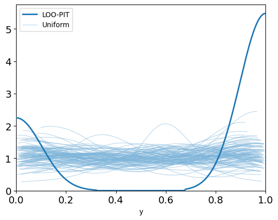
plot_loo_pit(idata_angle; y="y")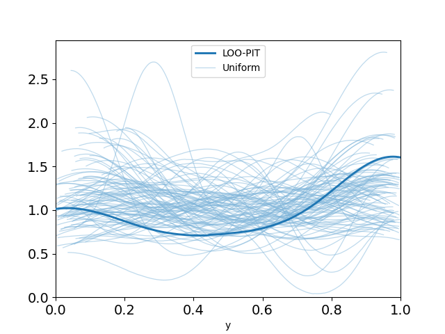

This looks pretty promising. Our LOO-PIT seems to be uniform. However, when we look at the ECDF plot we can see there's some difference between our estimate and the uniform CDF.

plot_loo_pit(idata_angle; y="y",ecdf=true)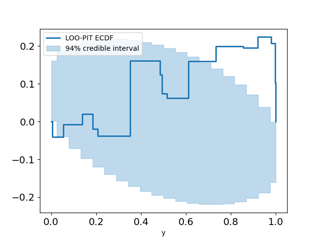

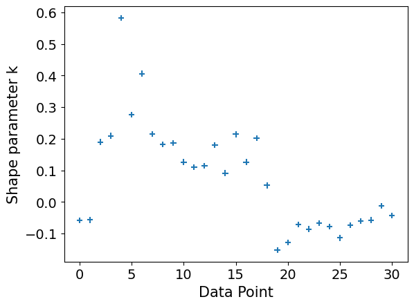
We also have one problematic Pareto $k$ value, rendering our estimate unreliable anyhow.

plot_khat(logistic_loo)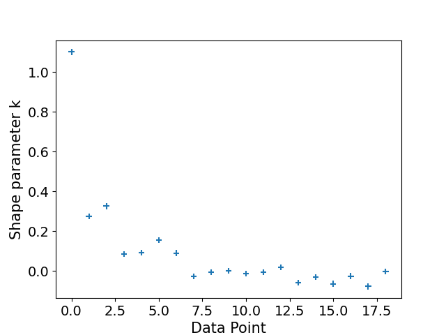

If this wasn't enough to convince you that the model isn't great, there is actually a lot more golf data available to us. Here I'll do something slightly different to the Stan documentation, and fit our model directly to this new data, to see how it performs.

data_new = readdlm("_assets/blog/golf-putting-in-turing/code/golf_data_new.txt")
x_new, n_new, y_new = data_new[:,1], data_new[:,2], data_new[:,3];
y = y_new./n_new
yerror_new = sqrt.(y .* (1 .-y)./n_new);

angle_model = golf_angle(x_new,y_new,n_new,r,R)
fit_angle = sample(angle_model,NUTS(),MCMCThreads(),2000,4)

Chains MCMC chain (2000×13×4 Array{Float64, 3}):

Iterations        = 1001:1:3000
Number of chains  = 4
Samples per chain = 2000
Wall duration     = 0.72 seconds
Compute duration  = 0.67 seconds
parameters        = sigma
internals         = lp, n_steps, is_accept, acceptance_rate, log_density, hamiltonian_energy, hamiltonian_energy_error, max_hamiltonian_energy_error, tree_depth, numerical_error, step_size, nom_step_size

Summary Statistics
  parameters      mean       std      mcse   ess_bulk    ess_tail      rhat   ess_per_sec
      Symbol   Float64   Float64   Float64    Float64     Float64   Float64       Float64

       sigma    0.0473    0.0000    0.0000   759.4126   1158.0842    1.0067     1128.3991

Quantiles
  parameters      2.5%     25.0%     50.0%     75.0%     97.5%
      Symbol   Float64   Float64   Float64   Float64   Float64

       sigma    0.0473    0.0473    0.0473    0.0473    0.0473

# get posterior median
med_sigma = quantile(Array(fit_angle),0.5)

threshold_angle = asin.((R-r) ./ x_new)
plot(x_new,2 .* cdf.(Normal(),threshold_angle ./ med_sigma) .- 1,color=:blue,linewidth=1.5)
scatter!(x_new,y, yerror = yerror_new,
        ylabel = "Probability of success",
        xlabel = "Distance from hole (feet)",
        title = "New data, old model",
        legend=:false,
        color=:lightblue)

And this really sends our posterior checks wild:

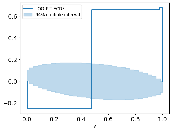
Something is definitely not right here, and it's clear that this data can't be explained only by angular precision. Indeed, in golf you can't just hit the ball in the right direction – you also have to hit it with the right amount of power^[5].

📝 The intuition for this next step in extending the model is much clearer if we plot the new data on top of the fit to the old data, as is done in the Stan documentation. I think this helps to illustrate that although posterior predictive checking can be very powerful, it shouldn't be the only thing you rely on.

An extended model that accounts for how hard the ball is hit

So we have an extra parameter now, sigma_distance, and additionally we make the assumption that the golfer aims to hit the ball 1 foot past the hole, with a distance tolerance of 3 feet (seriously if you're lost, read the Stan docs).

@model function golf_angle_distance_2(x,y,n,r,R,overshot,distance_tolerance)
    sigma_angle ~ truncated(Normal(),0,Inf)
    sigma_distance ~ truncated(Normal(),0,Inf)

    threshold_angle = asin.((R-r) ./ x)

    p_angle = 2 .* Phi.(threshold_angle ./ sigma_angle) .- 1
    p_distance = Phi.((distance_tolerance - overshot) ./ ((x .+ overshot) .* sigma_distance)) -
        Phi.(-overshot ./ ((x .+ overshot) .* sigma_distance))
    p = p_angle .* p_distance

    for i in 1:length(n)
        y[i] ~ Binomial(n[i],p[i])
    end
    return sigma_angle*180/π
end

overshot = 1
distance_tolerance = 3

angle_distance_2_model = golf_angle_distance_2(x_new, y_new, n_new, r, R, overshot, distance_tolerance)
fit_angle_distance_2 = sample(angle_distance_2_model,NUTS(),MCMCThreads(),2000,4)

Chains MCMC chain (2000×14×4 Array{Float64, 3}):

Iterations        = 1001:1:3000
Number of chains  = 4
Samples per chain = 2000
Wall duration     = 16.96 seconds
Compute duration  = 16.91 seconds
parameters        = sigma_angle, sigma_distance
internals         = lp, n_steps, is_accept, acceptance_rate, log_density, hamiltonian_energy, hamiltonian_energy_error, max_hamiltonian_energy_error, tree_depth, numerical_error, step_size, nom_step_size

Summary Statistics
      parameters      mean       std      mcse   ess_bulk   ess_tail      rhat   ess_per_sec
          Symbol   Float64   Float64   Float64    Float64    Float64   Float64       Float64

     sigma_angle    0.0311    0.0163    0.0041    21.6681   297.5836    1.9513        1.2812
  sigma_distance    0.0958    0.0356    0.0088    17.9589    23.4185    2.7383        1.0619

Quantiles
      parameters      2.5%     25.0%     50.0%     75.0%     97.5%
          Symbol   Float64   Float64   Float64   Float64   Float64

     sigma_angle    0.0132    0.0133    0.0342    0.0473    0.0473
  sigma_distance    0.0439    0.0794    0.0928    0.1369    0.1380

A bad fit

Now before we go jumping into our posterior predictive checks to try and confirm that our idea was as brilliant as we thought it was, let's take a quick look at the diagnostics provided by Turing. The ESS is very low and the $\hat{R}$ values for both parameters are much larger than 1, indicated poor mixing. We can plot the chains to see if we can see anything obvious.

plot(fit_angle_distance_2)

The chains are definitely not mixing, and it looks like they are getting stuck in some really tight local minima. The issue is with the Binomial error model, it tries too hard to fit the first few points (due to the $n_j$ being large) and this causes the rest of the fit to be off.

📝 Again, this illustrates that we don't always need posterior predictive checks to tell us if something is wrong. In fact, if the problem is obvious, as is the case here, we don't really need to go through all the effort of setting up the checks.

A good fit

The solution given is to approximate the Binomial data distribution with a Normal and then add independent variance. This forces (helps?) the model to not fit so well to certain data points to the detriment of others, improving the overall fit.

@model function golf_angle_distance_3(x,y,n,r,R,overshot,distance_tolerance)
    sigma_angle ~ truncated(Normal(),0,Inf)
    sigma_distance ~ truncated(Normal(),0,Inf)    
    sigma_y ~ truncated(Normal(),0,Inf)

    threshold_angle = asin.((R-r) ./ x)
    p_angle = 2 .* Phi.(threshold_angle ./ sigma_angle) .- 1
    p_distance = Phi.((distance_tolerance - overshot) ./ ((x .+ overshot) .* sigma_distance)) -
        Phi.(-overshot ./ ((x .+ overshot) .* sigma_distance))
    p = p_angle .* p_distance

    for i in 1:length(n)
        y[i] ~ Normal(p[i], sqrt(p[i] * (1 - p[i]) / n[i] + sigma_y^2));
    end
    return sigma_angle*180/π
end

angle_distance_3_model = golf_angle_distance_3(x_new,y,n_new,r,R,overshot,distance_tolerance)
fit_angle_distance_3 = sample(angle_distance_3_model,NUTS(),MCMCThreads(),2000,4)

Chains MCMC chain (2000×15×4 Array{Float64, 3}):

Iterations        = 1001:1:3000
Number of chains  = 4
Samples per chain = 2000
Wall duration     = 2.34 seconds
Compute duration  = 2.31 seconds
parameters        = sigma_angle, sigma_distance, sigma_y
internals         = lp, n_steps, is_accept, acceptance_rate, log_density, hamiltonian_energy, hamiltonian_energy_error, max_hamiltonian_energy_error, tree_depth, numerical_error, step_size, nom_step_size

Summary Statistics
      parameters      mean       std      mcse    ess_bulk    ess_tail      rhat   ess_per_sec
          Symbol   Float64   Float64   Float64     Float64     Float64   Float64       Float64

     sigma_angle    0.0178    0.0001    0.0000   3719.7112   4092.0236    1.0002     1613.0578
  sigma_distance    0.0801    0.0013    0.0000   3670.1854   3796.9313    1.0004     1591.5809
         sigma_y    0.0031    0.0006    0.0000   4050.1157   3588.2019    1.0015     1756.3381

Quantiles
      parameters      2.5%     25.0%     50.0%     75.0%     97.5%
          Symbol   Float64   Float64   Float64   Float64   Float64

     sigma_angle    0.0176    0.0177    0.0178    0.0179    0.0180
  sigma_distance    0.0776    0.0792    0.0800    0.0809    0.0827
         sigma_y    0.0020    0.0026    0.0030    0.0034    0.0044

# get posterior median
med_sigma_angle, med_sigma_distance, _ = [quantile(Array(fit_angle_distance_3)[:,i],0.5) for i in 1:3]

threshold_angle = asin.((R-r) ./ x_new)

p_angle = 2 .* Phi.(threshold_angle ./ med_sigma_angle) .- 1
p_distance = Phi.((distance_tolerance - overshot) ./ ((x_new .+ overshot) .* med_sigma_distance)) -
    Phi.(-overshot ./ ((x_new .+ overshot) .* med_sigma_distance))
post_line = p_angle .* p_distance

plot(x_new,post_line,color=:blue,legend=:false)

scatter!(x_new,y, yerror = yerror_new,
        ylabel = "Probability of success",
        xlabel = "Distance from hole (feet)",
        title = "Angle and distance model (good fit)",
        legend=:false,
        color=:blue)

So far so good. The moment of truth:

# Instantiate the predictive model
angle_distance_3_predict = golf_angle_distance_3(x_new,similar(y, Missing),n_new,r,R,overshot,distance_tolerance)
posterior_predictive = predict(angle_distance_3_predict, fit_angle_distance_3)

# Ensure the ordering of the loglikelihoods matches the ordering of `posterior_predictive`
loglikelihoods = pointwise_loglikelihoods(angle_distance_3_model, fit_angle_distance_3)
names = string.(keys(posterior_predictive))
loglikelihoods_vals = getindex.(Ref(loglikelihoods), names)
# Reshape into `(nchains, nsamples, size(y)...)`
loglikelihoods_arr = permutedims(cat(loglikelihoods_vals...; dims=3), (2, 1, 3));

idata_distance = from_mcmcchains(
    fit_angle_distance_3;
    posterior_predictive=posterior_predictive,
    log_likelihood=Dict("ll" => loglikelihoods_arr),
    library="Turing",
    observed_data=(; y)
);
distance_loo = loo(idata_distance,pointwise=true);
println("LOO is ",round(distance_loo.elpd_loo[1],digits=2), " with an SE of ",round(distance_loo.se[1],digits=2),
        " and an estimated number of parameters of ",round(distance_loo.p_loo[1],digits=2))

LOO is 127.33 with an SE of 5.04 and an estimated number of parameters of 5.06

plot_loo_pit(idata_distance; y="y")
plot_loo_pit(idata_distance; y="y",ecdf=true)
plot_khat(distance_loo)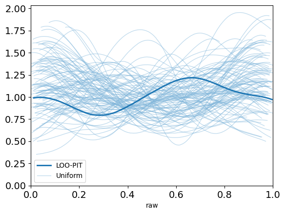

Model selection

One final thing we can do, although it's more or less redundant in this example, is to compare our models based on PSIS-LOO. In order to do this we can use the compare function. It takes a Dict of InferenceData objects as input, and returns a DataFrame ordered from best to worst model.

📝 Some of our models were fit to different datasets – to do model comparison that actually makes sense, the different models have to be fit to the same data. I won't show the code for this but the models have been re-fit to the new data.

comparison_dict = Dict("logistic" => idata_logistic,
                       "angle" => idata_angle,
                       "angle_distance_3" => idata_distance)
compare(comparison_dict)

3×10 DataFrame
 Row │ name              rank   elpd_loo        p_loo        elpd_diff  weight       se           dse      warning  scale
     │ String            Int64  Float64         Float64      Float64    Float64      Float64      Float64  Bool     String
─────┼─────────────────────────────────────────────────────────────────────────────────────────────────────────────────────
   1 │ angle_distance_3      0     127.326         5.06047         0.0  1.0              5.04021      0.0     true  log
   2 │ logistic              1  -72580.1        2941.02        72707.4  0.0          15950.1      15951.1     true  log
   3 │ angle                 2      -1.90037e5     0.158715   190164.0  8.42231e-11  67980.4      67978.3     true  log

Conclusion

If you've been wanting to do posterior predictive checks with your models in Turing and didn't know where to start, hopefully you've learnt something from this post and will be able to integrate these tools into your workflow.

Thank you to all the hard work of the Turing and ArviZ developers, as well as everyone I've referenced here, and thanks to Jo Kroese for helping me with the CSS, so now the images are actually big enough to see.

References

[1]	https://jduncstats.com/posts/2019-11-02-golf-turing/

[2]	Practical Bayesian model evaluation using leave-one-out cross-validation and WAIC. https://arxiv.org/abs/1507.04544v5

[3]	https://oriolabrilpla.cat/python/arviz/pymc3/2019/07/31/loo-pit-tutorial.html

[4]	Using the loo package (PSIS diagnostic plots). https://mc-stan.org/loo/articles/loo2-example.html

[5]	Anyone who's played Wii Sports Resort golf knows this all too well.